
Fire simulations in the EVAC platform are created using information from a variety of sources. Learn more about how the simulations are created with this guide.
Fire Model
Genasys's fire simulations are based on ELMFIRE (Eulerian Level Set Model of Fire Spread) developed by Chris Lautenberger. For details about the model see Lautenberger, 2013. To create fire simulations, ELMFIRE requires a variety of landscape, fuel, and weather data inputs along with user-defined parameters that control spotting rate of the fire.
Data
ELMFIRE requires weather, landscape and topography, and fuel inputs. The following section describes data inputs and their sources in greater detail.
Weather
All weather inputs are listed below:
-
relative humidity
-
temperature
-
wind speed
-
wind direction
|
Data |
Source |
Description |
Resolution |
|---|---|---|---|
|
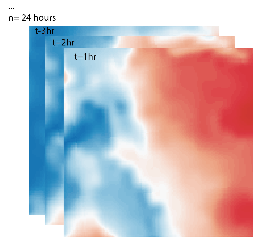
Weather Forecasts |
Weather forecasts are hosted by Pyregence. The 24-hr forecasts are based on the High Resolution Rapid Refresh model (HRRR), which is a WRF based forecast modeling system. Forecasts are updated every 6-hrs |
spatial resolution=3 km by 3 km
temporal resolution = 1 hr |
|
|
Historical Weather |
If historical weather is selected to simulate a fire, the closest station to the ignition point that has wind speed, wind direction, relative humidity, and temperature record is used for the weather record. If some of the record is missing, data is linearly interpolated.
|
Data is not spatially distributed. For fire simulations less than 12 hours, data is aggregated at half hour time-step using median values. For fires over 12-hrs, data is aggregated to 1-hr time steps (to reduce computational time) |
|
|
Extreme Weather |
Hard-coded values:
|
Currently extreme weather is modeled using uniform values to represent strong, hot, and dry winds that originate over the desert and blow from the east. Santa Ana and Diablo winds are an example on the west coast. |
Data is not spatially distributed. Data is not temporally distributed (same weather values during the entire simulation). Simulation time-step is 1-hr (having finer resolution does not significantly affect simulated perimeters) |
Landscape
All landscape fuel and topography inputs are listed below. For detailed description of the landscape fuel layers, see https://landfire.gov/fuel.php
-
Canopy Base Height
-
Canopy Bulk Density
-
Canopy Height
-
Canopy Cover
-
Aspect
-
Digital Elevation Model (DEM)
-
40 Fire behavior Fuel Models Scott/Burgan
-
Slope
-
Non-burnable mask (see “Burnable areas” section)
|
Data |
Source |
Description |
|---|---|---|
|
LANDFIRE |
30 m by 30 m resolution data available for the entire United States. Currently 2016 remap data is used for all fuel layers with the exception of the “40 Fire behavior Fuel Models Scott/Burgan” for which a 2020 remap is used. |
Note: we do not use historical fuel models; for all historical weather, regardless of year, 2016/2020 LANDFIRE fuel maps are used
Fuel Moisture
All fuel moisture inputs are listed below:
-
Live herbaceous fuel moisture
-
Live woody fuel moisture
-
1-hour dead fuel moisture
-
10-hour dead fuel moisture
-
100-hour dead fuel moisture
Fuel moisture is divided into moisture content of live (herbaceous and woody) and dead (1-hr, 10-hr, and 100-hr) fuels. For dead fuels, the name of the fuel corresponds to the time (longer time = bigger/thicker fuel) it takes for fuel moisture to equilibrate with changing atmospheric conditions.
In preparation for a fire simulation, fuel moisture is calculated by numerically integrating first order ordinary differential equation which is a function of fuel’s moisture equilibrium content, instantaneous moisture content, and time lag. Fuel’s moisture equilibrium content is a function of relative humidity and temperature. These calculations rely on relative humidity and temperature only. Precipitation is not currently accounted for. For more details about how fuel moisture is calculated, see Lautenberger 2013. Fires simulated within the Zonehaven platform are initialized with the fuel moisture content of 6%, 7%, and 8% for 1-hr, 10-hr, and 100-hr fuels respectively across all weather conditions with the exception of the extreme weather, where fuel moisture calculations is initialized with 2%, 4%, and 6% for the same fuel categories.
Burnable areas
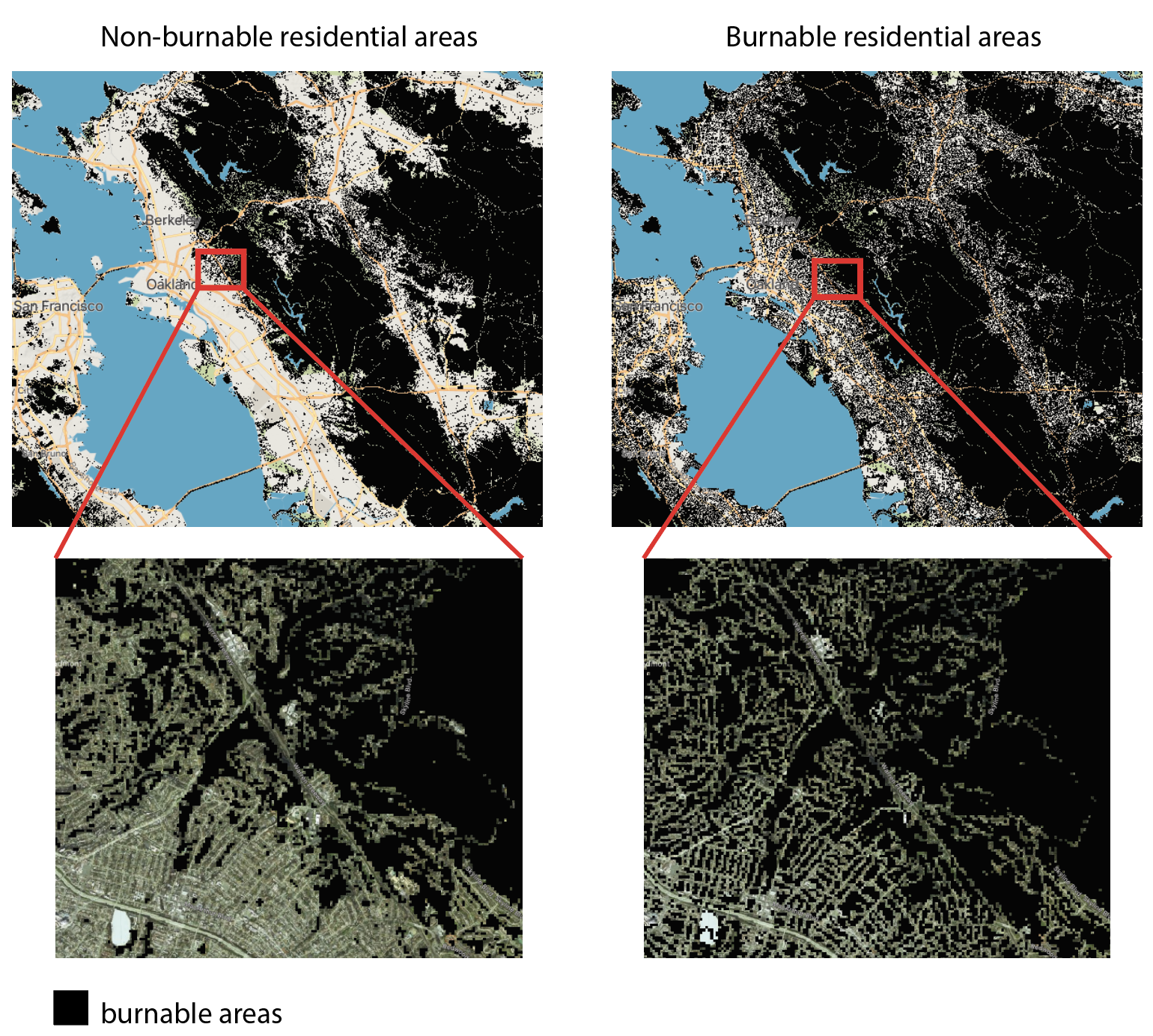
Not all areas can burn. In the example of the city of Oakland, CA, dense downtown areas are unlikely to burn. However, residential low density housing in the Oakland Hills is interspersed with dense vegetation and is very likely to catch on fire. In fact, large areas of the Oakland Hills did burn in the Oakland Hills Fire of 1991.
LANDFIRE classifies all urban/residential areas as “urban” fuel type, which is considered non-burnable by ELMFIRE (left panel in the figure below). Genasys has altered LANDFIRE’s fuel map to make low to medium density residential areas to be considered burnable by the fire spread model. Meanwhile high density areas and major roads remained non-burnable. See the right panel of the figure below.
Spotting
Using ELMFIRE algorithms, surface and crown spotting can be produced for all pixels containing a passive or active crown fire. One percent of all burning surface and crown pixels produces an ember, and that ember has a 50% probability of being ignited (20% if extreme weather; see section Spotting: Extreme Weather).
Spotting distance (x) itself is calculated probabilistically from a lognormal distribution. Mean spotting distance (m) and its variance (v) are related to 20-ft wind speed (u20) as:
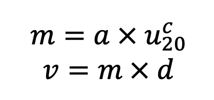
where a, c, and d are parameters that influence the spotting distance distribution. In the future, these parameters will be calibrated to specific regions, but currently they are set to a=5, c=0, and d=100.
The normalized mean (mu) and standard deviation (sigma) of the lognormal distribution are then calculated from m and v as:
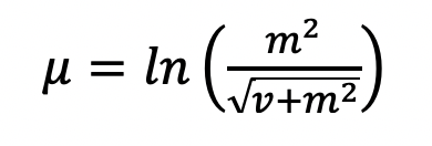
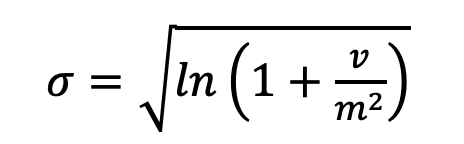
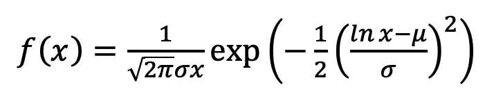
Spotting distance (x) is calculated probabilistically from a lognormal distribution:
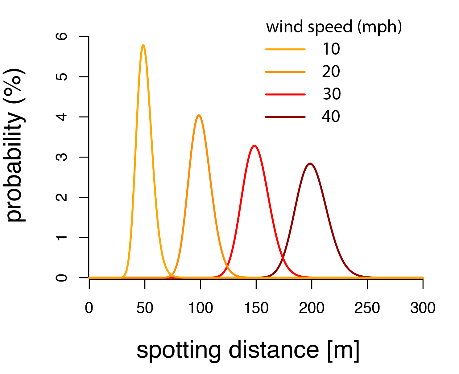
The figure below shows the spotting distance probability for different wind speeds. Generally, as wind speed increases, spotting distance increases as well, but the probability distribution gets wider too.
Spotting: Extreme Weather
When extreme fire weather (wind speed of 30 mph) or custom weather with wind speeds above 25 mph are used, spotting and fire spread parameters are altered in the following ways:
-
probability of ignition of an ember is changed from 50% to 20%
-
fire spread rate (unitless) is tripled
-
critical spotting fireline intensity is increased from 0 to 1500 kW/m (only applies to surface spotting)
Above changes were made to decrease computational time by reducing the number of spot ignitions while maintaining the overall fire size.
If a combination of high wind speeds (above 25 mph), densely vegetated areas without barriers (roads, rivers, rock-outcrops), and long fire duration (10+ hours), is used to model a fire, it is possible that simulations will take over an hour.
Avoid these simulations, since it is highly unlikely that extreme wind speeds will be sustained the entire time-period and thus the fires will not be realistic.